Spoken Digit Recognition

Objective

The objectives of this project are to train an ML model with the spoken digit training dataset so that it accurately classifies spoken digits that the model has not previously encountered, as well as identify and justify design tradeoffs. Different modeling decisions will be compared to show how they impact results.

Spoken digit recognition is used in automated phone calls, car navigation systems, and other environments where hands-free dictation is convenient. Additionally, the problem of spoken digit recognition can be extended to general speech recognition, which is used in translation, subtitle generation, speech-to-text, and similar applications.

In addition to speech recognition, the modeling process pursued in this project is relevant to other problems that rely on classification, such as autonomous driving. In autonomous driving systems, before the vehicle can make decisions it first has to understand the world around it. This involves classifying obstacles in its environment, including vehicles, pedestrians, traffic signals, and roads. Models must train on vast amounts of data in order to accurately classify people and objects in the world around it. In this scenario, accuracy is critical for the safety of vehicle occupants as well as pedestrians and other drivers.

Data Modeling

The complete dataset has 8800 total spoken digits, or 880 samples of each digit. The full dataset is split into a training set of 6600 samples (660 per digit) and a testing set of 2200 samples (220 per digit).

Each sample is a processed audio recording. This processing involves converting the audio into a time series for 13 Mel Frequency Cepstral Coefficients (MFCCs).^{[2], [3]} Each sample is a “block” of data, and each block is made of frames. A frame is an array of 13 MFCC values at a certain point in time.

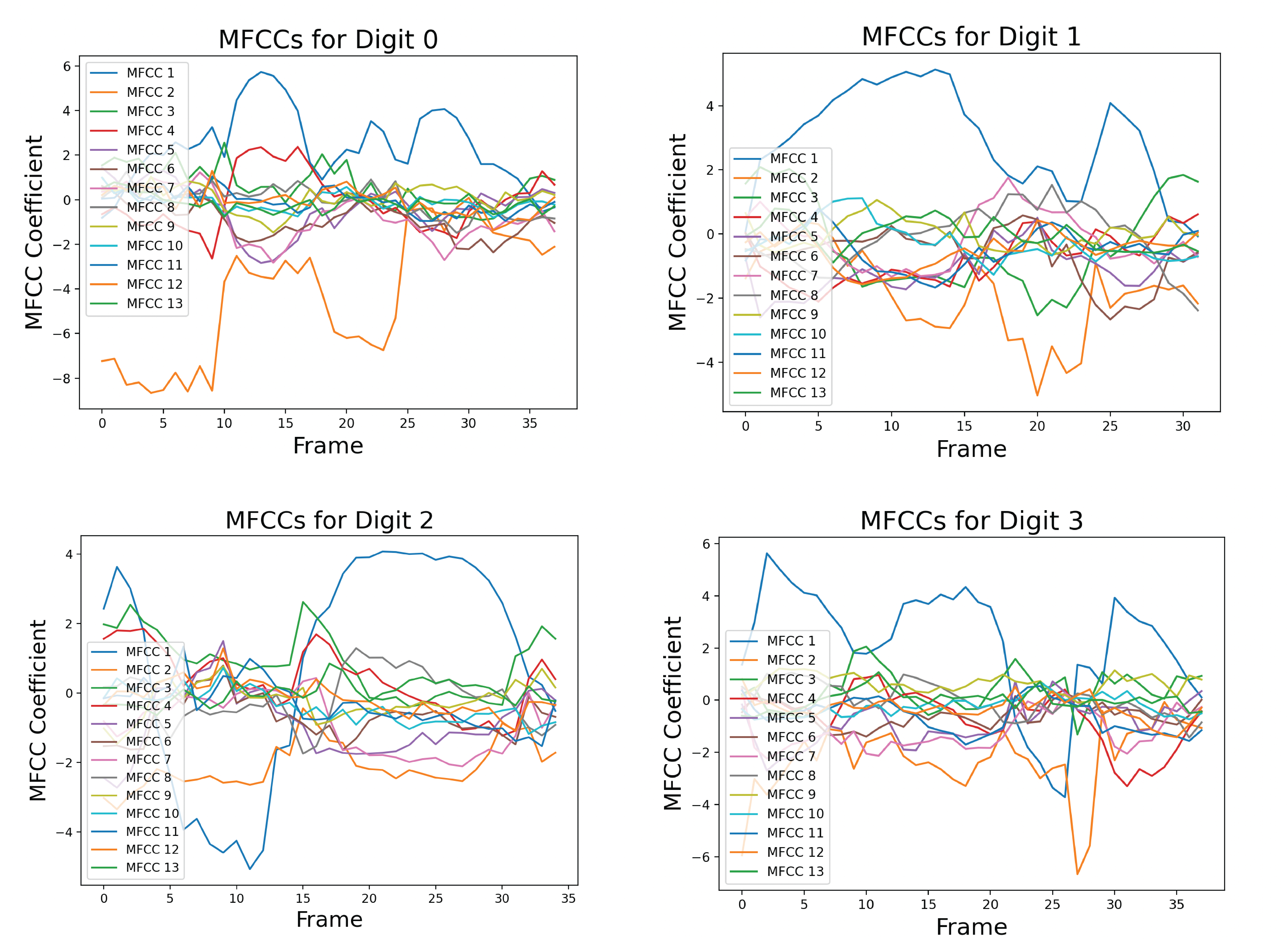
The above images show the MFCCs for one sample of the spoken digits zero, one, and two. Each sample, or block, can have a different number of frames, usually between 30 and 40.

For each block, the time series of MFCCs can be broken down into chunks. These chunks are called phonemes, and they represent distinct sounds made by the speaker. Phonemes can be identified by the magnitude of MFCC coefficients, as well as the relation of the MFCCs with one another. Digits usually have three or four, and they are highlighted below.

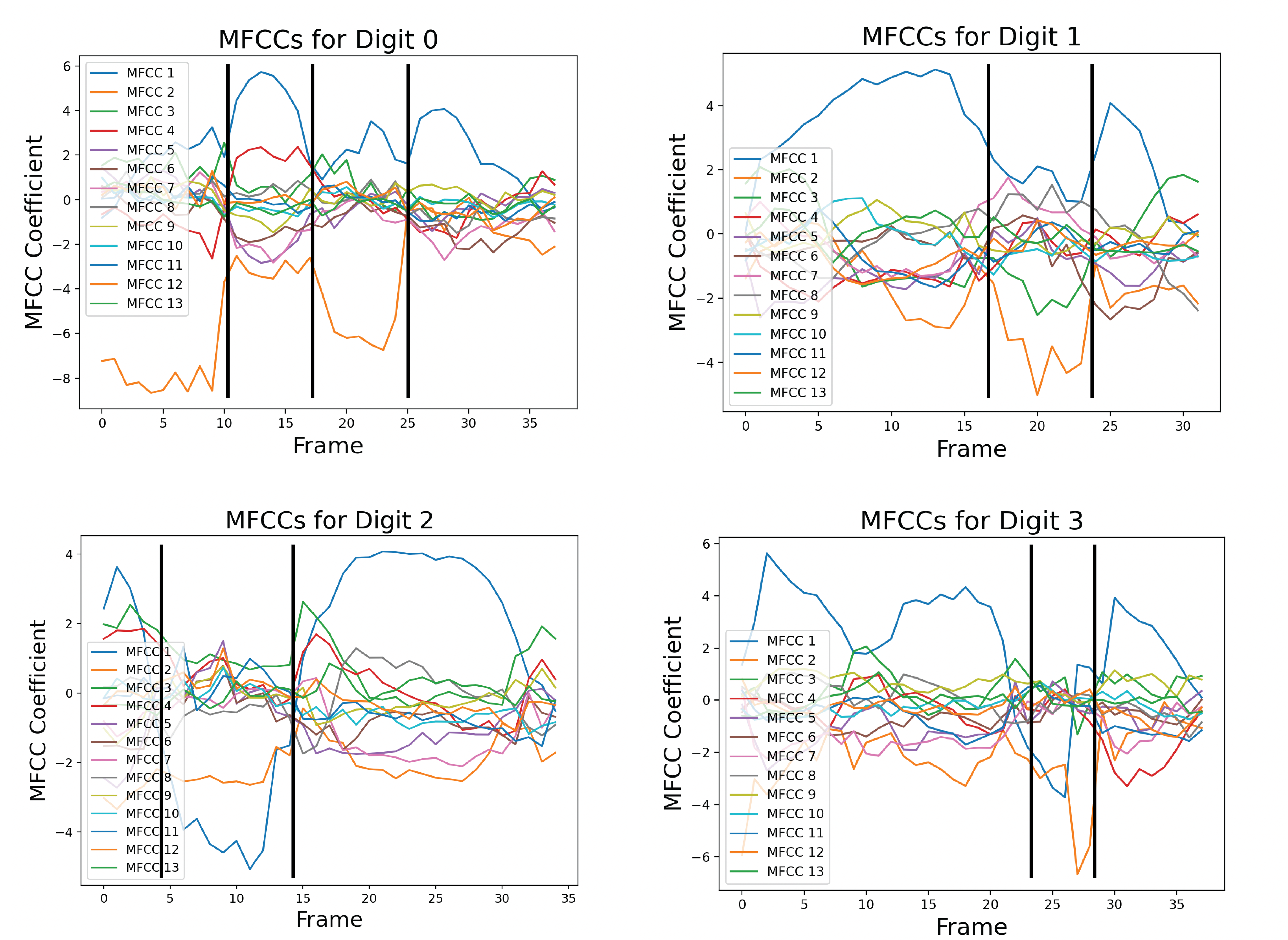
Each sample will have slightly different coefficient strengths for the same phonemes, as each speaker has a different voice. This can be visualized as scatter plots between different MFCCs for a digit.

Some MFCCs group together with others, but some may have little or no correlation with each other. The key takeaway from this visualization is that different digits have different phonemes, and different phonemes have different distributions of MFCCs. Additionally, while these scatter plots compare two dimensions of MFCCs, there are really 13 MFCCs that create a 13-dimension cluster for each phoneme.

Knowing that digits have different sets of identifiable phonemes, it makes sense to want to find phonemes and quantify their parameters – means and covariances – using the data. If the data is arranged into clusters of points that can be labeled together as a phoneme, then a model can be created that classifies new data based on the phonemes that it matches with.

K-Means

One approach that takes the data and groups it together is called k-means clustering. K-means is a machine learning algorithm that starts out with K number of means (usually randomly chosen) and iterates over all of the data to find the mean that is closest to each data point. It sorts the data into K groups, each corresponding to one of the K means. After every point is added to a group, the group mean is recalculated, and then the algorithm repeats.^[6]

For this problem, because digits have three or four phonemes, k-means clustering will be performed with k equal to three and four, with results being compared. Additionally, the number of iterations of k-means will be varied, and distance between points will be calculated using Euclidean distance.

The means themselves begin as randomly generated arrays with 13 elements corresponding to the 13 MFCCs for each frame. “Distance” is the difference between the MFCC values for a frame and the mean MFCC values. The goal of k-means is to minimize the distance between every frame and its cluster's mean. In order to perform k-means on a digit, all of the frames from all of the blocks of that digit are used to create clusters. This minimization is performed for every iteration of k-means. This can be expressed with the following equations^[4]:

$$ \min_{C_1, ... , C_K} \sum_{k=1}^{K} \sum_{x\in{}C_k}||x-\mu_k||^2 $$ $$ \mu_k = \frac{1}{|C_k|} \sum_{ x \in{} C_k} x $$

The first equation is the expression that k-means aims to fulfill. The clusters \(C_1\) to \( C_K \) are chosen so that the sum of the distances between every point in each cluster and the cluster's mean is minimized. This means that every point has been assigned to the cluster closest to it. The second equation defines the cluster mean, \(\mu_k \), simply as the average value of all the frames, \( x \), in the cluster \(C_k \). This is calculated at the end of an iteration of k-means, when the first equation has been fulfilled. This updates the cluster mean for the next cycle of k-means, which will affect how the first equation is satisfied during the next iteration.

Below are the cluster assignments for the MFCCs. Again, these clusters exist in 13 dimensions, so two-dimensional slices of the full cluster are used to visualize the cluster shape between MFCCs. This causes some points to appear as if incorrectly assigned to a cluster in 2D, when in 13D they are correctly assigned.

After clustering with k-means, it is useful to define a distribution for each cluster. This distribution is assumed to be Gaussian for each cluster, with \( x \) being a frame and \( C_k \) being a cluster.

$${p(x|C_k) = \mathcal{N}(x | \mu_{k}, \Sigma_{k})}$$

Each cluster has its own mean, \( \mu_{k} \), and covariance matrix, \( \Sigma_{k} \) that define the Gaussian for that cluster. K-means computes the means, but the covariance matrices need to be calculated using the points in each cluster.^[4]

There are different kinds of covariance matrices that can be used for the GMM. A spherical covariance matrix assumes that every variable - in this case every MFCC - is independent and has no covariance with other MFCCs. This results in a matrix where only the diagonal is non-zero and every diagonal element is equal. A diagonal matrix also assumes no covariance between variables, but the variance for each MFCC may be different. Finally, a full covariance matrix assumes nothing about the independence of variables, resulting in a matrix that is “full” of nonzero values.

Apart from assumptions about covariance, each of the spherical, diagonal, and full matrix types can either be distinct or tied. Choosing distinct covariance matrices means calculating a different matrix for each cluster using the data from that cluster. Contrastingly, choosing to use a tied covariance matrix means calculating a single covariance matrix using all of the data from all clusters. Thus, every Gaussian distribution will have the same covariance matrix.

These plots show different GMMs based on choice of K, the number of clusters. As a result of using more clusters, more computation is required each iteration to find the closest cluster mean. Digits with four phonemes can be characterized more accurately by creating four clusters, but digits with three phonemes would work better with three clusters. This is a tradeoff between computation and accuracy, as well as accuracy for individual digits. For these plots, distinct full covariance matrices were used. The effects of different types of covariance will be explored in the next section.

A different way to model the data is by creating a separate GMM for male and female speaks for each digit. Each GMM will be built with 330 samples, plotted here:

This modeling choice revealed that there is a big difference between the phoneme clusters for male and female speakers. This surprised me because I thought the phonemes would be roughly the same. There is less data available for each cluster, but the Gaussians fit the data better than those for the combined male-female models.

Expectation-Maximization

When using k-means clustering to find phonemes, the covariance matrices were calculated at the end of the algorithm. The k-means clusters were created using only the means of the clusters, but what if covariance could be taken into account during clustering?

Expectation-maximization (EM) is a method that iterates over each point and determines which cluster it should belong to based on the probability of a point belonging to a cluster, the cluster mean, and the cluster covariance. This is the likelihood that the point belongs to a given cluster. Rather than minimizing distance as in k-means, EM maximizes likelihood of a point belonging to a cluster.^[5]

$$ k_x = \arg\max_{k} [\pi_k \mathcal{N}(x | \mu_{k}, \Sigma_{k})]$$

The likelihood is expressed by \( \pi_k \mathcal{N}(x | \mu_{k}, \Sigma_{k}) \) and is the probability of a point being in the cluster multiplied by the distribution of that cluster. The value of \( k_x \), which corresponds to a cluster, is chosen so that the frame \( x \) has the greatest likelihood of being in cluster \( k \).^[4]

For every round of EM, \( k_x \) is computed for every \( x \), creating clusters. After all the frames have been clustered, these following equations^[4] update the model parameters, the probability, mean, and covariance for each cluster. \( n \) is simply the total number of frames in the EM problem.

$$ n = \sum_{ k = 1 }^{K} |C_k| $$ $$ \pi_k = \frac{1}{n} |C_k| $$ $$ \mu_k = \frac{1}{|C_k|} \sum_{ x \in{} C_k} x $$ $$ \Sigma_k = \frac{1}{|C_k|} \sum_{ x \in{} C_k} (x - \mu_{k}) (x - \mu_{k})^T$$

The covariance matrix, mean, and probability for each cluster are calculated in every iteration, starting at random or pre-defined values. The results are clusters that may be shaped more like Gaussian distributions opposed to the clusters defined by distance as in k-means. The covariance matrix is a 13-by-13 matrix that contains the variance of each MFCC on the diagonal, and all the covariances of MFCCs with each other throughout the rest of the matrix.

Here are cluster assignments made with EM using distinct full covariance matrices, shown side-by-side with cluster assignments made by k-means.

While the full shape of the EM clusters cannot easily be assessed through this visualization, it shows the difference between the two clustering methods. K-means clustering more clearly groups points that are close in space, while EM clusters points that together form a Gaussian shape.

EM clusters change shape based on the type of covariance matrix used during clustering.

From top to bottom, the plots are ordered by increasing flexibility and computational effort, from tied spherical to distinct full matrices. As covariance flexibility increases, the Gaussian distributions better match the shape of their clusters. This leads to increased model complexity, or closeness to the training data, however this does not necessarily translate to accurate predictions for testing data.

Notice how the tied and distinct spherical covariance matrices closely resemble the k-means classifications. Because the variance in all directions of a spherical covariance are equal, the likelihood of a point belonging in that cluster decreases with Euclidean distance. As the complexity of the covariance increases, the Gaussians capture more of the cluster shape.

Another aspect of EM is the use of cluster probability. This is calculated each iteration based on the number of points in a cluster divided by the total number of points. One side effect of using probability in the likelihood calculations is that clusters might “take over” and gain significantly more points within them. This is shown in the distinct diagonal and tied full covariance contour maps. Here are those GMMs plotted again without the use of probability in likelihood calculations:

Removing the probability in the likelihood calculations produces clusters with an even amount of data in each cluster. The modified likelihood equation is:

$$ k_x = \arg\max_{k} [\mathcal{N}(x | \mu_{k}, \Sigma_{k})]$$

The probability component of likelihood is removed, but the cluster mean and covariance are used to calculate the maximum cluster likelihood and assign each point to a cluster.

Maximum Likelihood Classification

After making a GMM for each digit, whether via k-means or expectation-maximization, it is possible to introduce a new sample to the model, calculate the likelihood that the sample is each digit, and choose the digit that produces the maximum likelihood^[4] as the predicted digit for the new data.

$$ d_X = \arg\max_d \Pi{}_{i=1}^{|X|} \max_{k\in{}d} [\pi_k \mathcal{N}(x_i | \mu_{k}, \Sigma_{k})]$$

The predicted digit \( d \) for sample \( X \) is the digit that maximizes the product of maximum cluster likelihoods. A maximum cluster likelihood is the greatest likelihood that a frame \( x_i \) of the sample \( X \) belongs in the cluster \( k \) of the digit \( d \).

Because the maximum cluster likelihoods may be small values, the product is at risk of underflow, or being set to zero due to rounding during computation. This can be solved by taking the log of likelihoods and computing the sum:

$$ d_X = \arg\max_d \sum{}_{i=1}^{|X|} \max_{k\in{}d} [\log{\pi_k} + \log{\mathcal{N}(x_i | \mu_{k}, \Sigma_{k})}]$$

This yields the same predicted digit as the first likelihood equation.

This is called maximum likelihood classification, as the testing sample is classified as the digit that produces the maximum likelihood value for that sample.

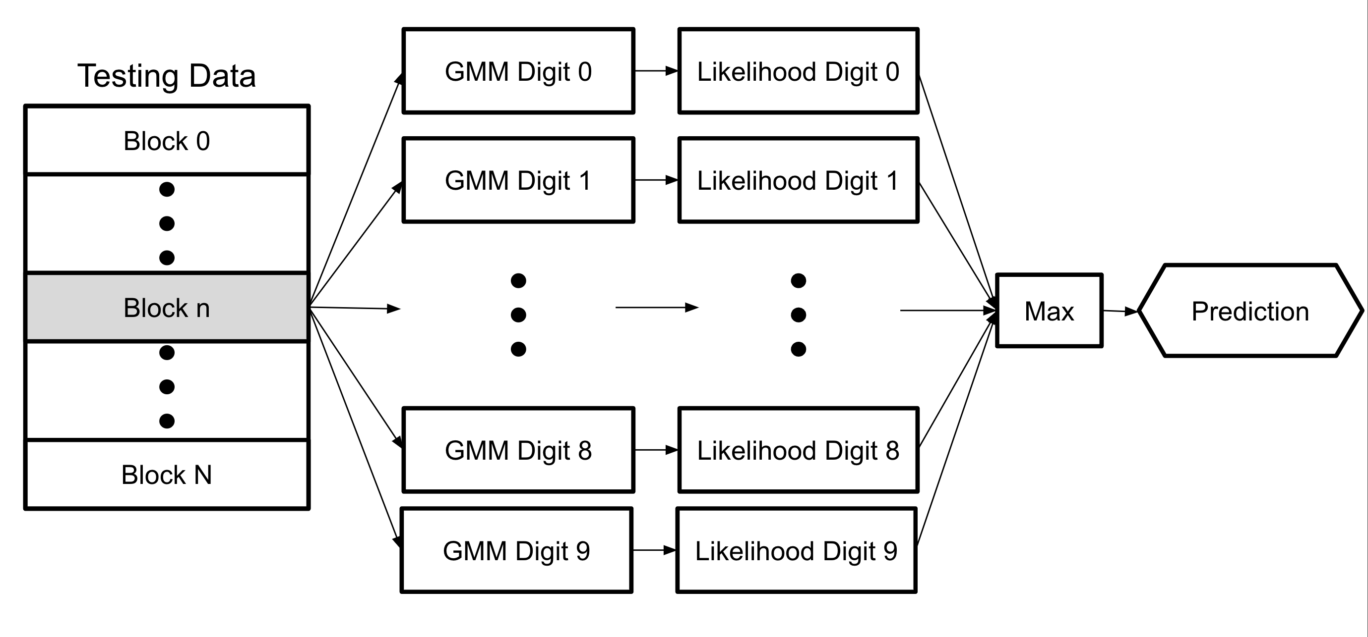
At a high level, each sample, or block, is passed into each GMM and the likelihood that the sample is each digit is output. After getting all ten digit likelihoods, the algorithm iterates over the likelihood values and uses the maximum likelihood to get the digit prediction for the testing sample.

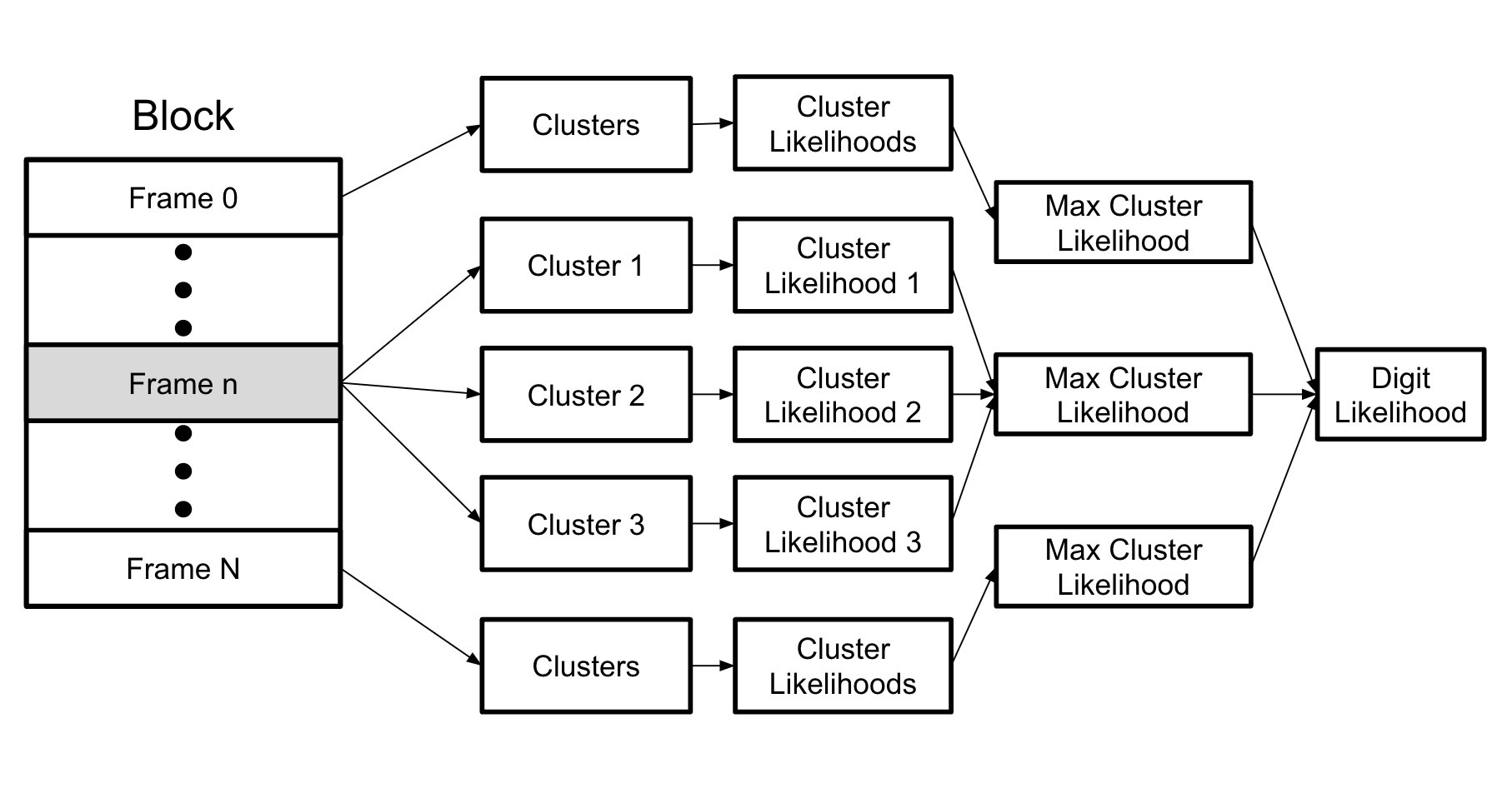
This chart shows a more detailed process for getting the likelihood that a single block is a single digit and GMM. One-by-one, frames are passed into the likelihood functions for the GMM. A likelihood value for the frame belonging to each cluster is returned. For each frame, the maximum cluster likelihood is selected. Finally, the maximum cluster likelihoods for each frame are either multiplied or the log of the likelihoods are added to get the total likelihood that a block is a specific GMM.

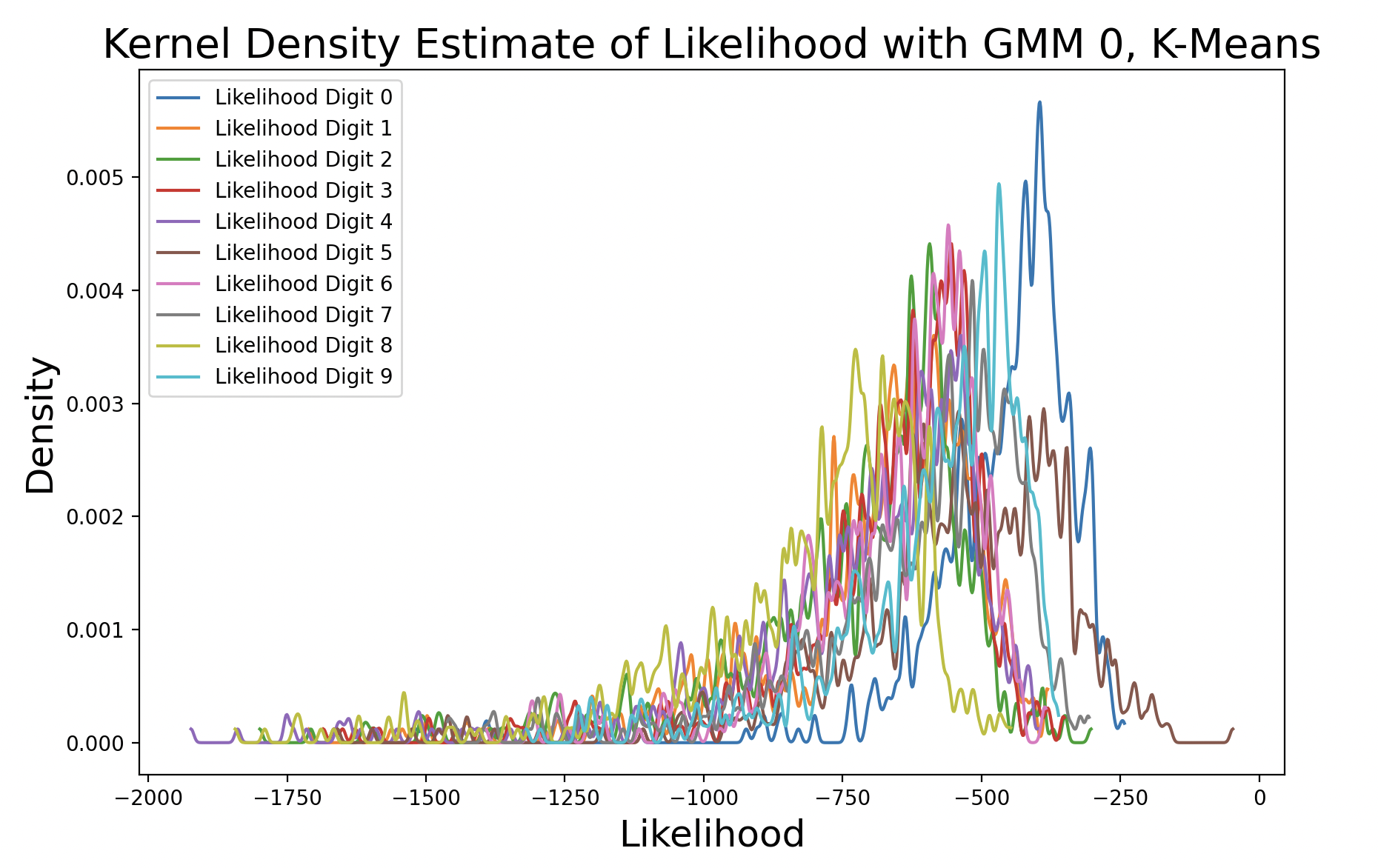
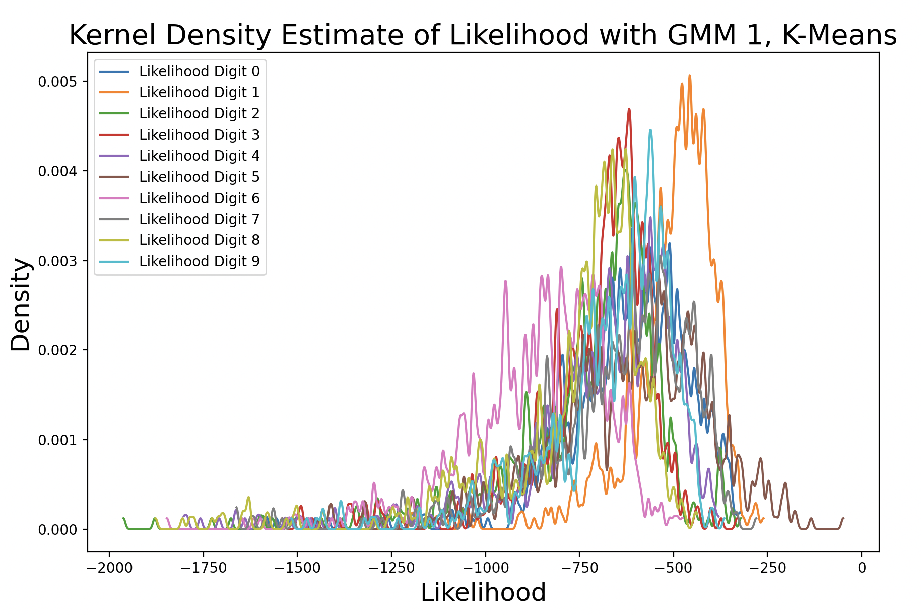
These plots show the likelihood of every (training) sample being the digits zero and one, respectively. The further to the right a likelihood is, the more likely that sample matches the GMM it was tested against. Both plots show the digit that matches the GMM with the highest density, meaning that predictions for that digit are the most consistent around the peak density. Additionally, the peak of the matching digit occurs the farthest to the right out of all of the kernel density curves. This indicates that with the greatest consistency, the matching digit will be the most likely condidate for the GMM.

A k-means model was used to get these density estimates. This model is not perfect, which is why in some cases the likelihood for incorrect digits exceeds that of matching digits. EM can also be used to create the GMM to perform this test. Here are the results with different distinct covariance matrices:

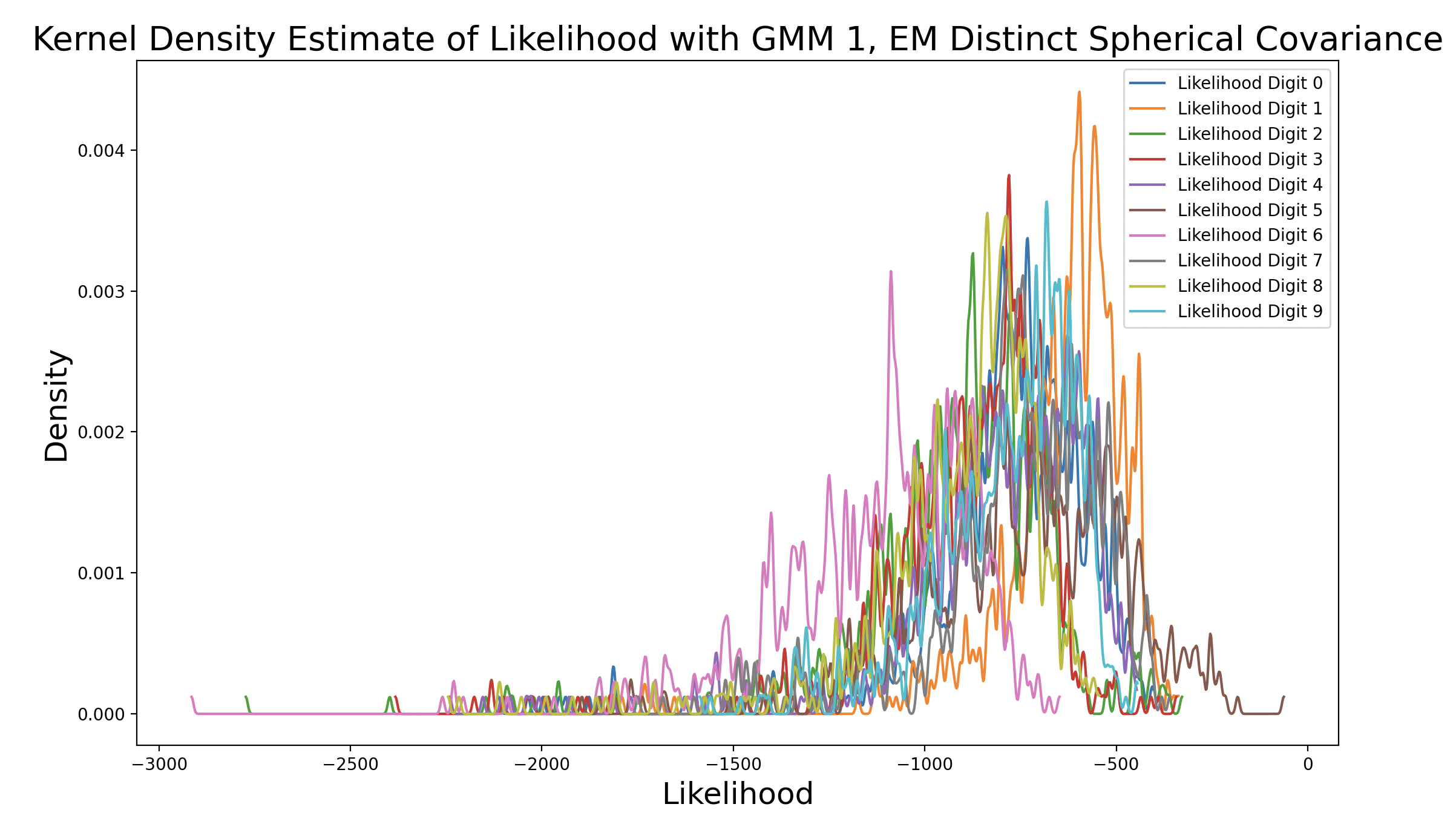
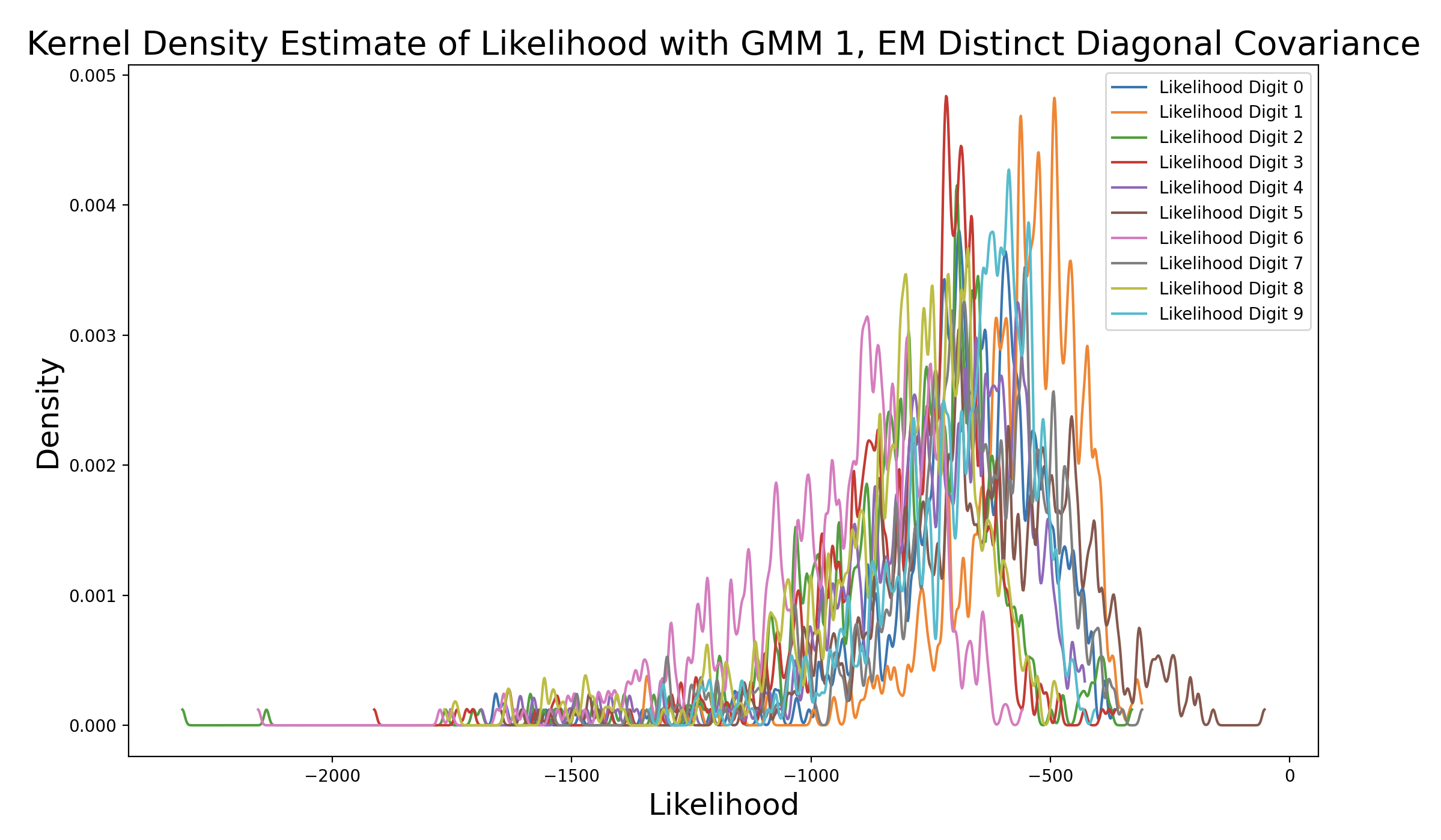
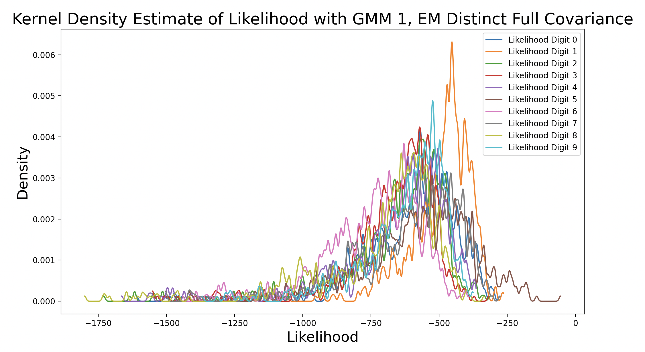
As the EM models increase in complexity due to changing covariance matrix type, the peak of the matching digit curve increases in height and shifts to the right of the plot. This means that the peak occurs at increasing levels of likelihood. Additionally, as the peak density increases, the consistency of likelihood estimates increases. The peak of the matching digit ends up taller than the other peaks in the final plot, indicating that the other likelihood estimates are more varied. This makes sense because only some of the other samples should produce high likelihoods (false predictions), while the rest are much lower. Interestingly, the peaks of other curves also increase with model complexity, although they still peak to the left of the matching digit. This could be because the more complex GMM captures the shape of certain phonemes well, so digits that share one or more phonemes with the true digit end up with higher likelihood estimates.

In order to expand this process to perform maximum likelihood classification, a GMM for each digit must be calculated. Then, testing data will be passed into each GMM. The maximum likelihood that results will give the prediction digit.

Maximum likelihood classification is useful for this problem because it uses the concept of maximum likelihood estimation for each digit individually, opposed to other prediction methods like maximum a posteriori (MAP), which requires an assumption about the prior. With this particular testing dataset, the distribution is uniform between each digit, so it is expected that maximum likelihood and MAP predictions are the same. Additionally, in the real world it would be difficult to make assumptions about the prior, so it is more beneficial to exchange the potential benefits of using a prior for faster compute times by maximizing only likelihood.

One way to display the model predictions of test data is a confusion matrix^[7]. Each row of a confusion matrix corresponds to the true digit of a sample, while the column is the prediction for that sample. For example, if a sample of the digit one is predicted to be a three, the confusion matrix would display “1” in row one, column three. This means that, ideally, the diagonals should have the largest values in their respective rows, indicating that the prediction is correct.

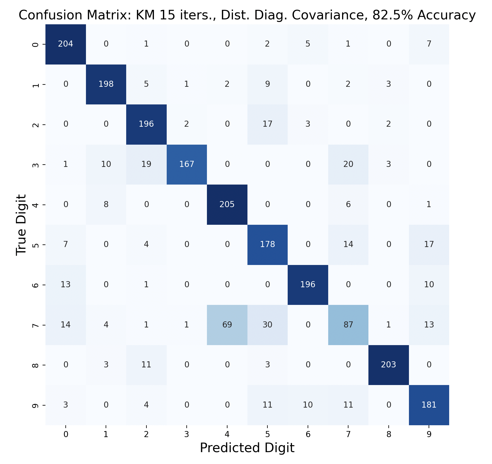
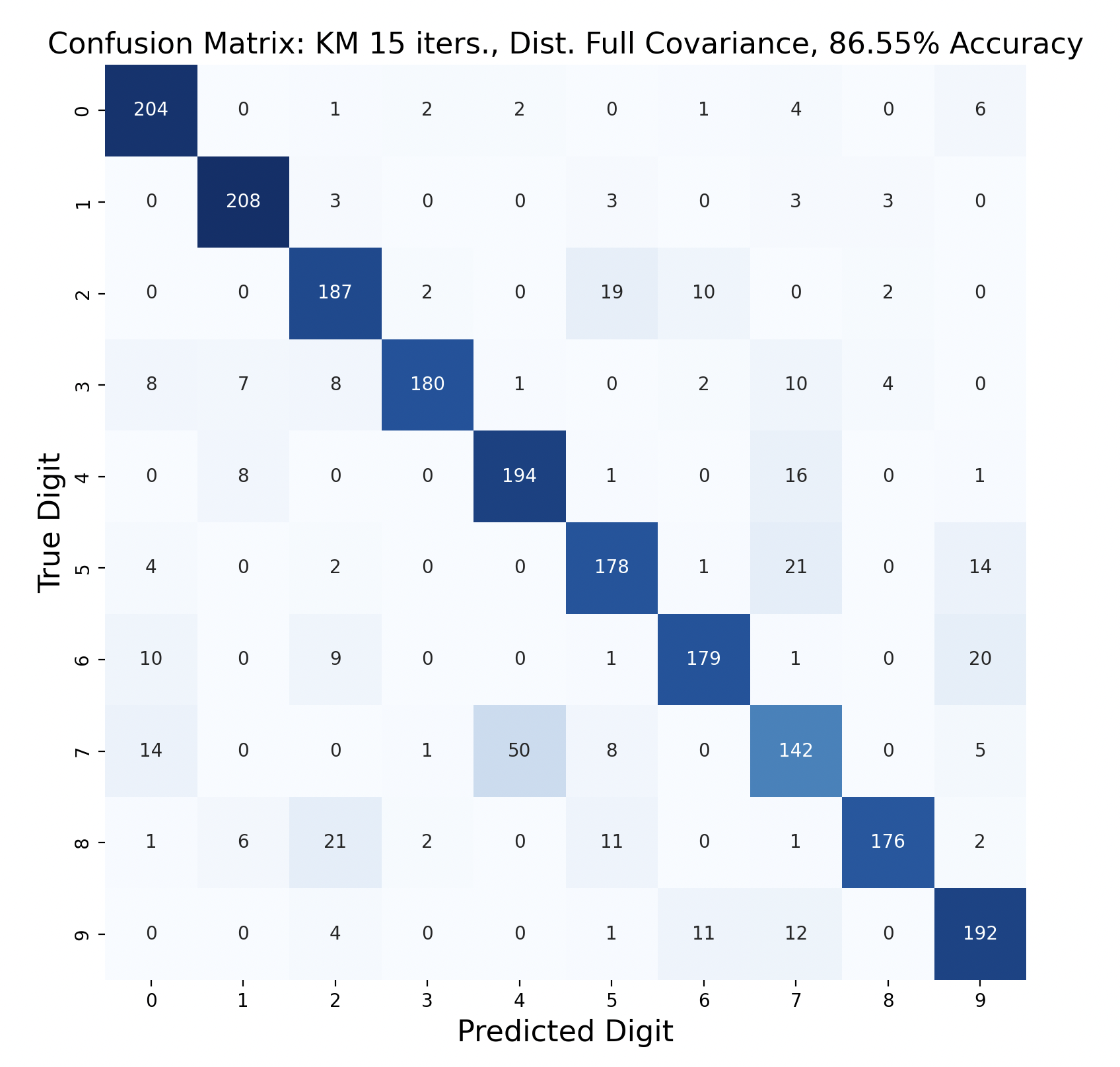
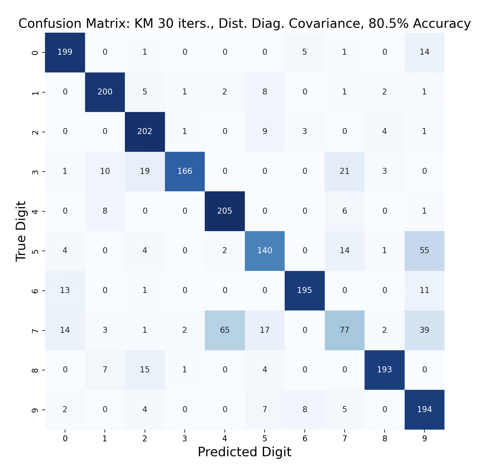
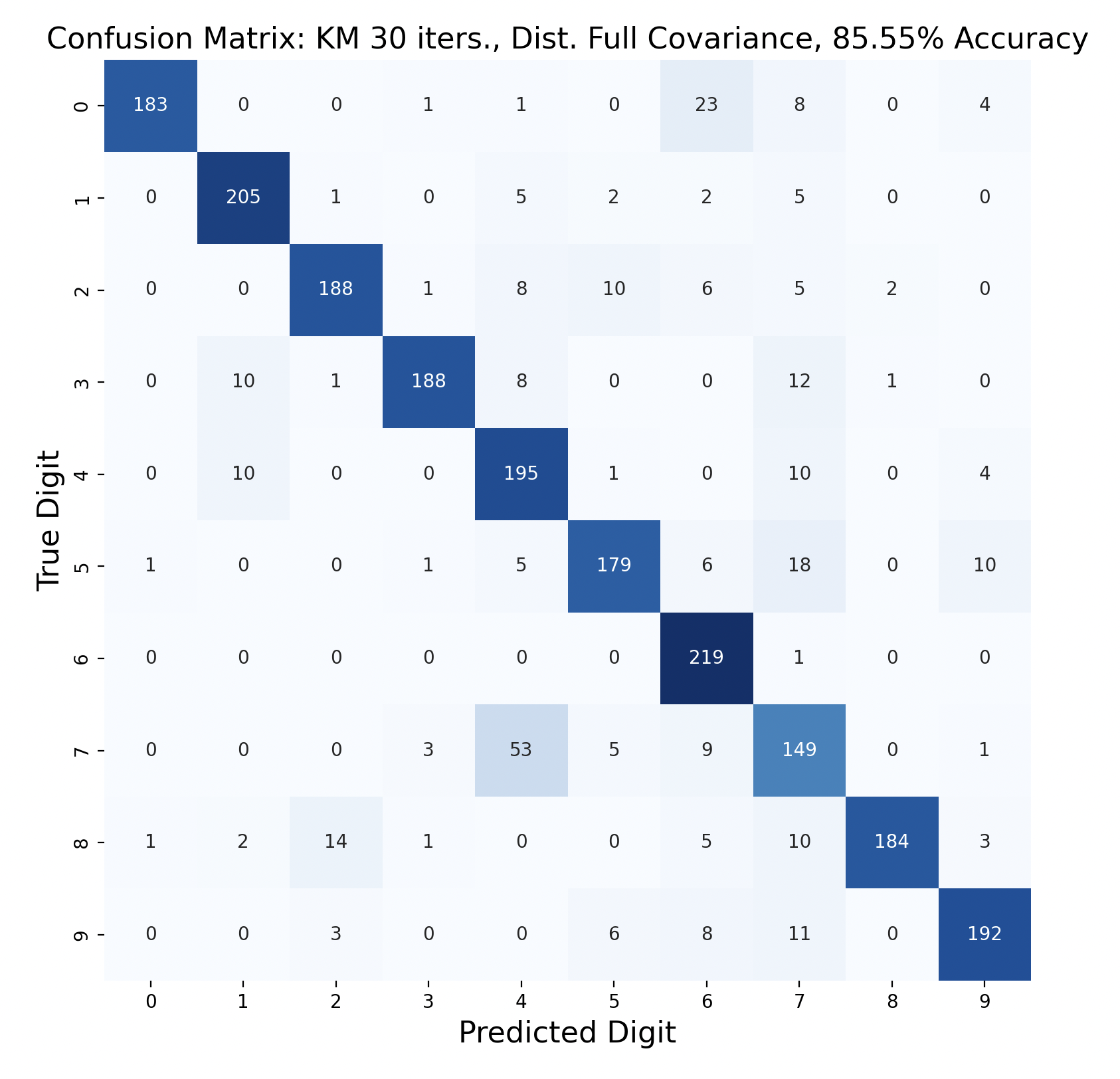
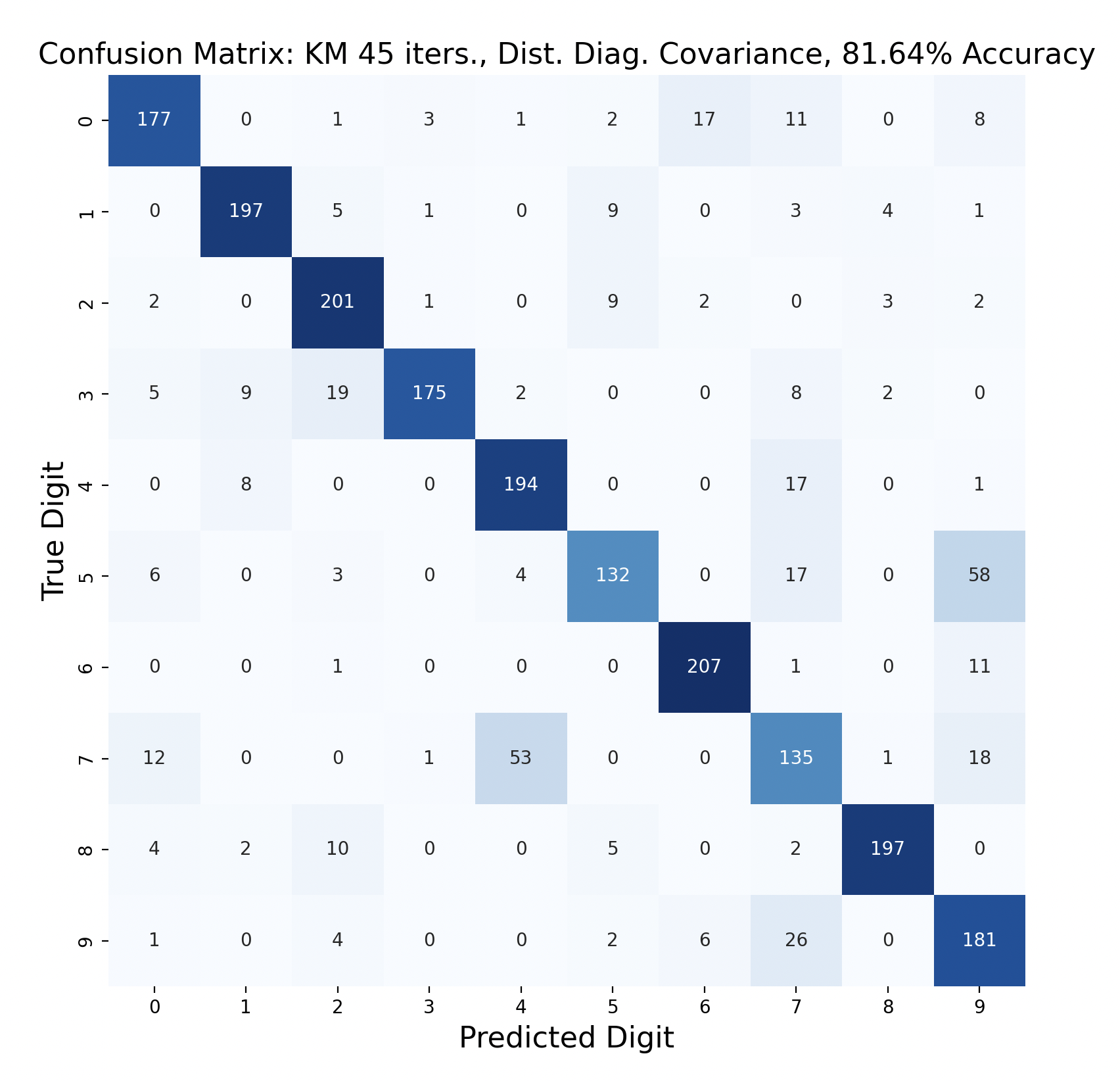
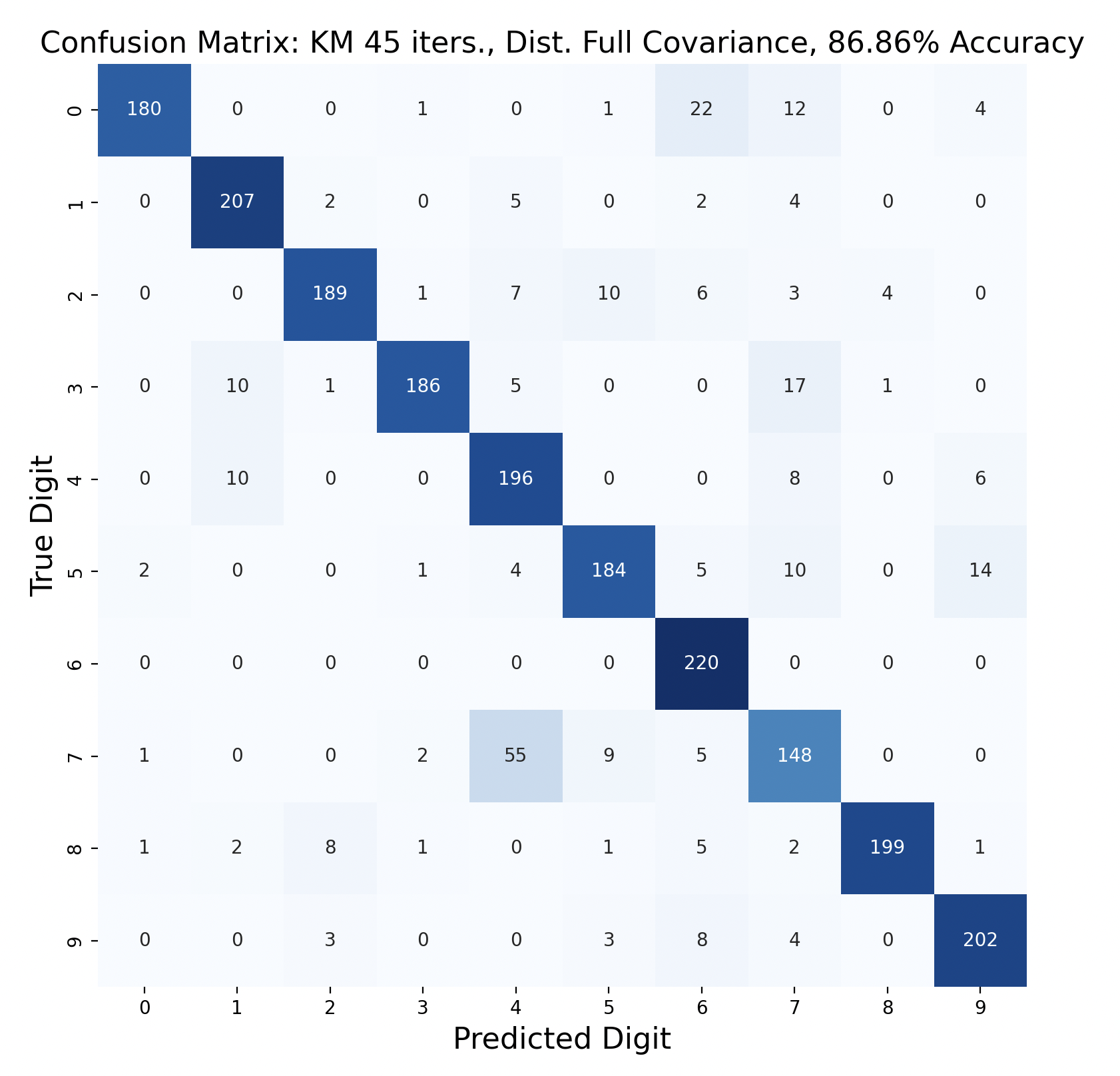
There are 2200 samples in the testing set, with 220 for each digit. The confusion matrices show the results of classifying the testing data via k-means but with varied iterations and covariance types. In each case, the diagonals have the largest values in their rows, however there are differences resulting in the variation of parameters between tests.

Out of these k-means maximum likelihood classification trials, the trial with the most iterations, 45, and full covariance matrices performed the best with an overall accuracy of 86.86%. At the other end, the worst performing test was with 30 iterations and distinct diagonal covariance matrices. Between both types of covariance matrices, there is increasing accuracy as the number of iterations increases. This means that these models are likely a bit biased, and model complexity can increase further before accuracy is lost.

For every number of iterations, the version with distinct diagonal matrices performed worse than the version with distinct full covariance matrices. This shows that the full covariance matrices, while better fitting the training data, also are better at classifying the testing data.

The models consistently performed well for digits one and six, with the most accurate model predicting six correctly for 100% of the testing samples.

Interestingly, digit zero performed well on the first few models with less iterations, but became one of the least accurate digits for the most accurate model. At the same time, the models with less iterations also incorrectly predicted zero a lot more often compared to the later models, showing that while zero became less accurate, this contributed to the entire model becoming more accurate.

The digit that was the least accurately predicted was seven, across every single model. When a seven was classified incorrectly, it was most often classified as a four, then as a nine. To gain insight as to why this is the case, the words for seven, four, and nine can be examined: “seb’a,” “araba’a,” and “tis’ah”. These words share similar ending sounds, which means that they share phonemes with each other. This leads to frames from seven having high likelihood matches with phoneme clusters of four and nine. Nine and four were also mistaken for seven, but not as often as the reverse. In general, seven was a popular incorrect prediction, and nine was a popular incorrect prediction particularly for distinct diagonal models.

Because accuracy increased with the number of iterations, and full covariance matrices performed better, the following are k-means trials with full covariance and increasing iterations:

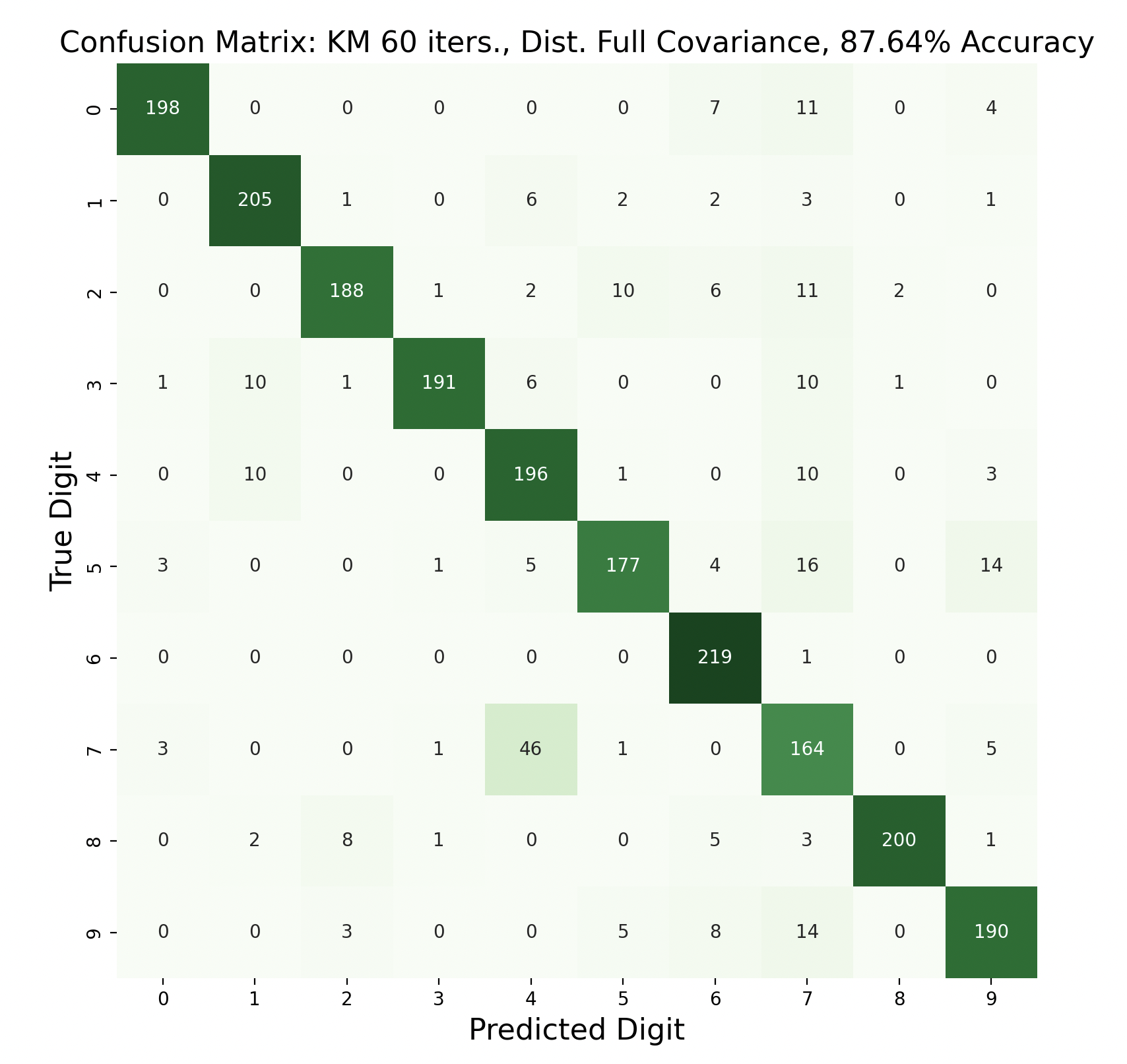
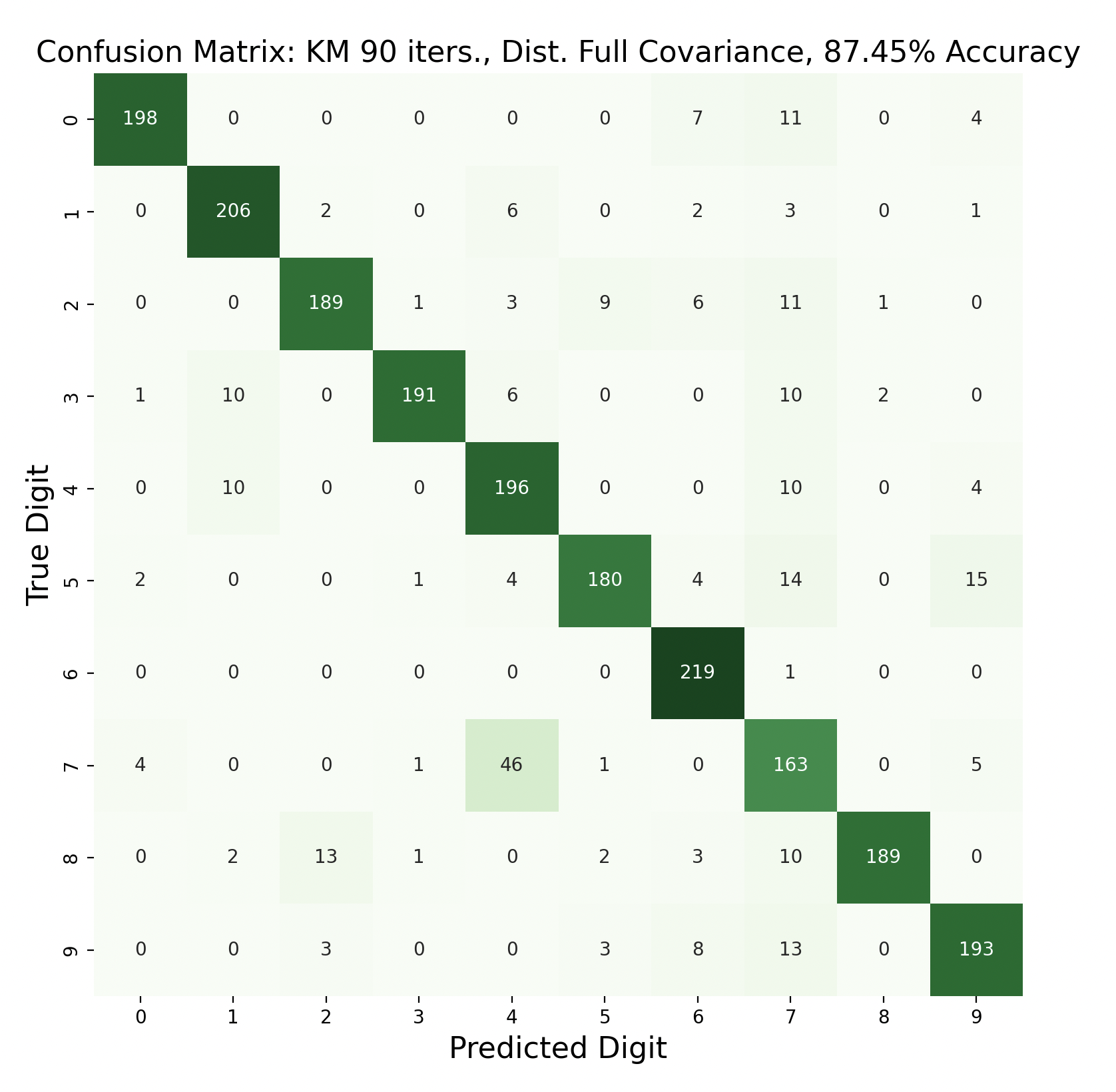
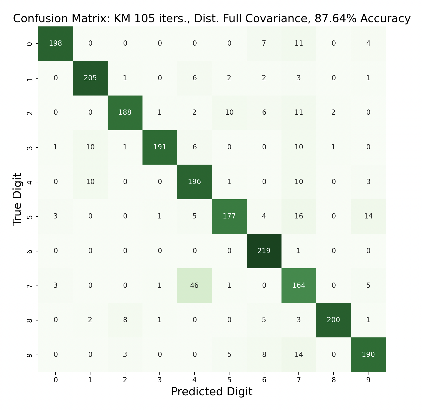
After increasing the number of iterations for k-means, the accuracy for the models peaked at 87.91% for 75 iterations before declining slightly. This shows that the clusters made by k-means converge after about 75 iterations. This means that the updated means don't cause any cluster restructuring, so the clusters and means remain the same and the resulting models are very similar in accuracy as a result.

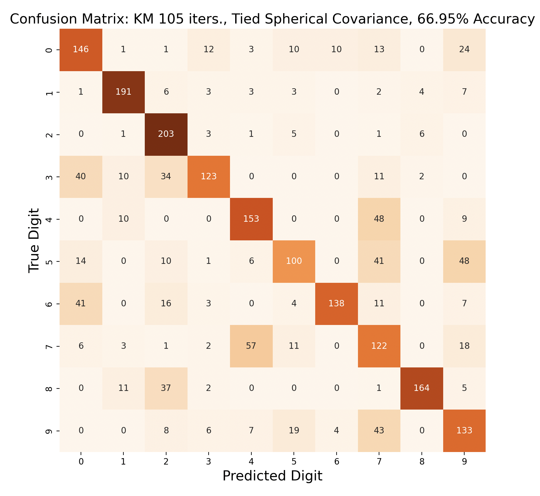
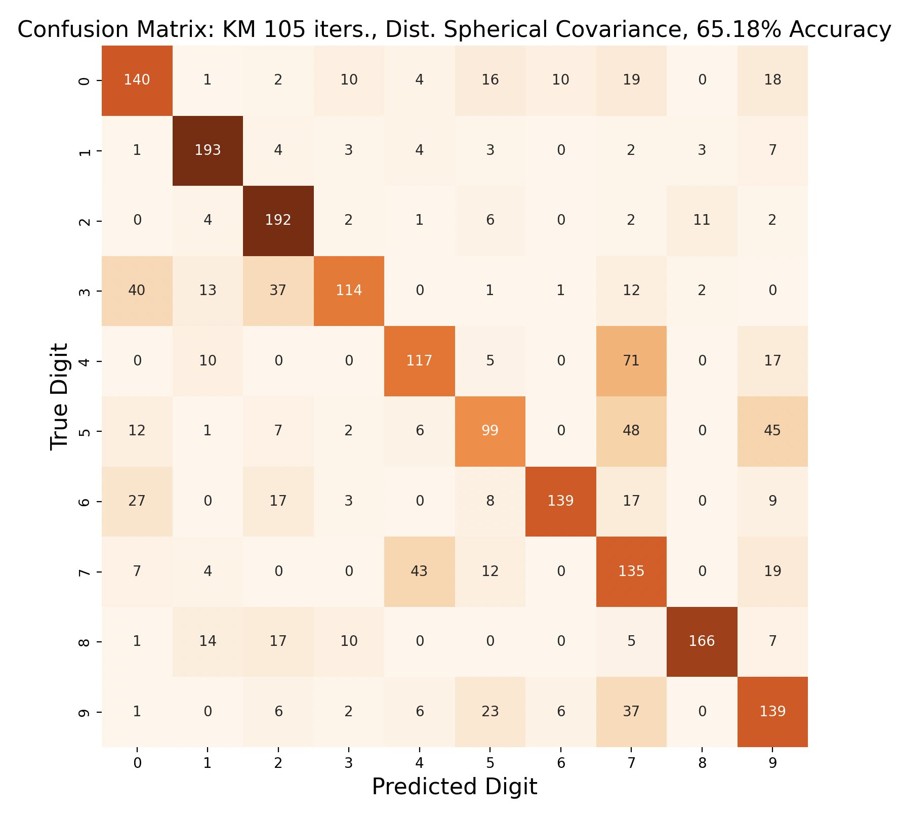
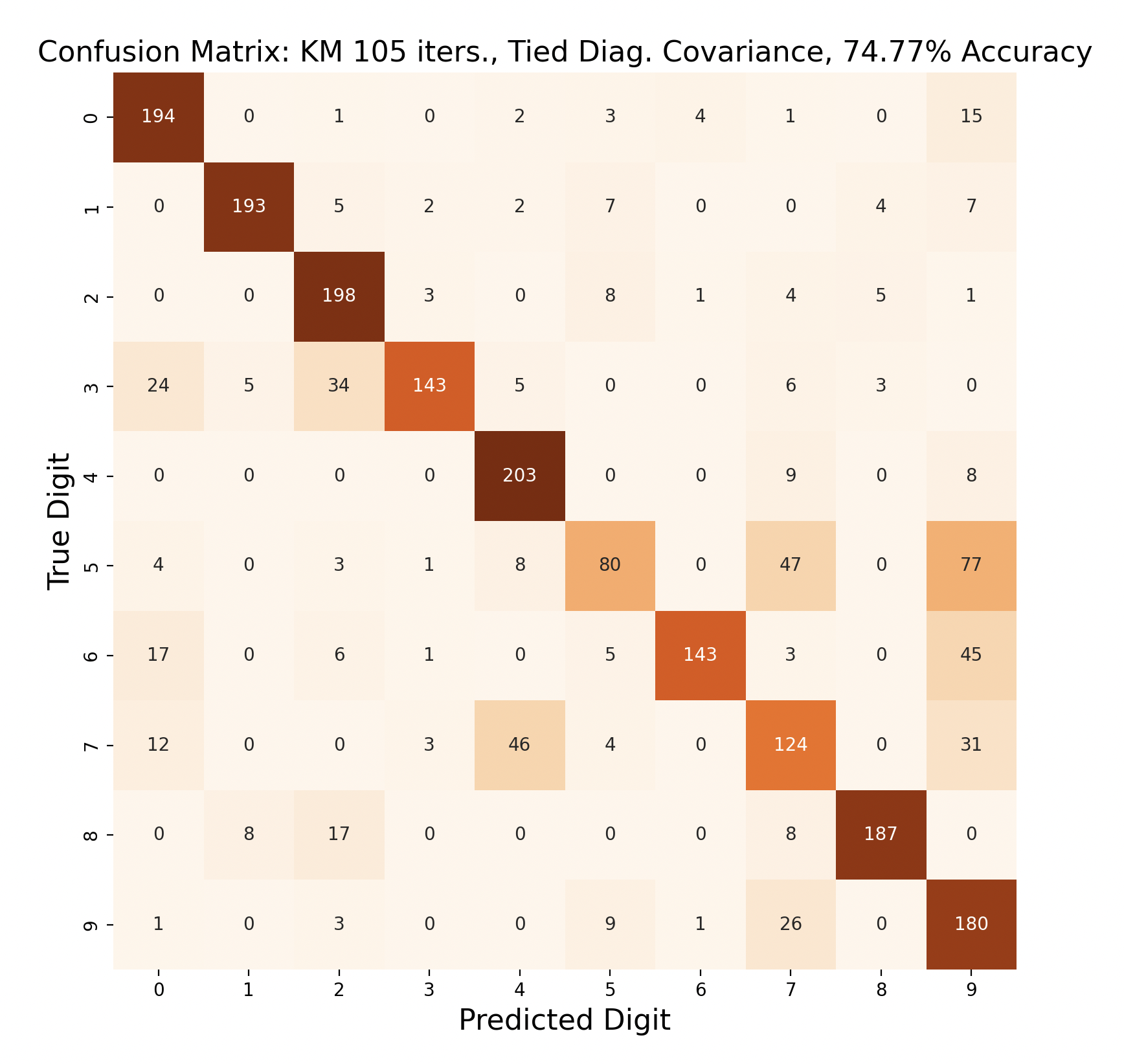
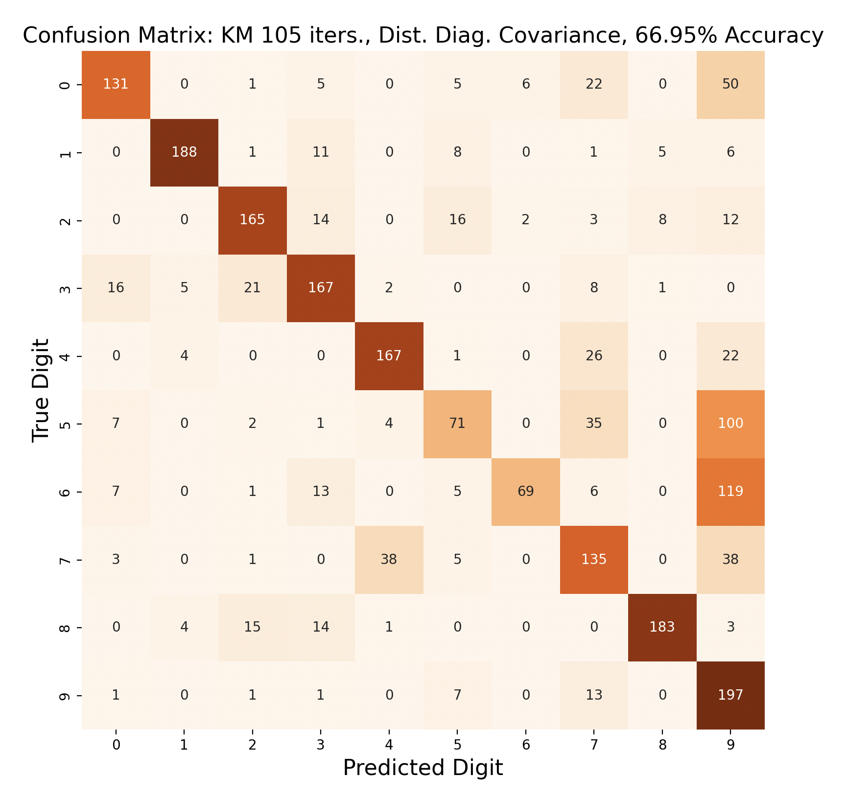
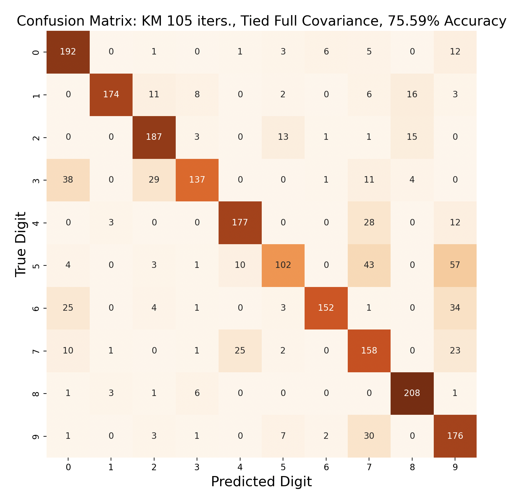
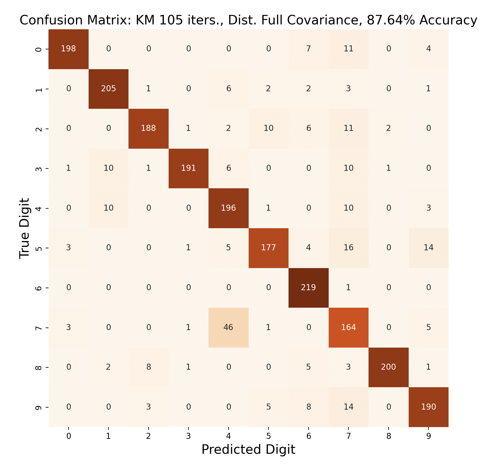
The above group of confusion matrices show the results and overall accuracy for a model built with k-means clustering. From top to bottom, the models increase in flexibility starting with tied spherical covariance and ending with distinct full covariance. For spherical and diagonal covariance models, the tied versions perform better than distinct versions. This surprised me as I thought having distinct matrices would always result in higher accuracy. This is only the case for full matrices. For the majority of covariance types, the models had trouble correctly identifying fives, sixes, and sevens. In the distinct full covariance model, six performed the best, but in all previous models it was one of the worst subproblems.

Another key observation is that the distinct diagonal model performed very poorly for 105 iterations of k-means, with an accuracy of 66.95%. This model actually classified five and six most often as nine than the correct digit. Compared to the 45 iteration distinct diagonal results (81.64% accuracy), it seems that for more rigid covariance types, it is beneficial to limit the number of iterations of clustering so that cluster assignments are not extremely tied to the data. When the shape of the diagonal covariance Gaussians are fit very closely to the data, they end up making more mistakes than the full covariance matrices.

GMMs created through expectation-maximization can also be used for maximum likelihood classification. Here are the results of test data classification with EM with varied number of iterations and types of covariance.

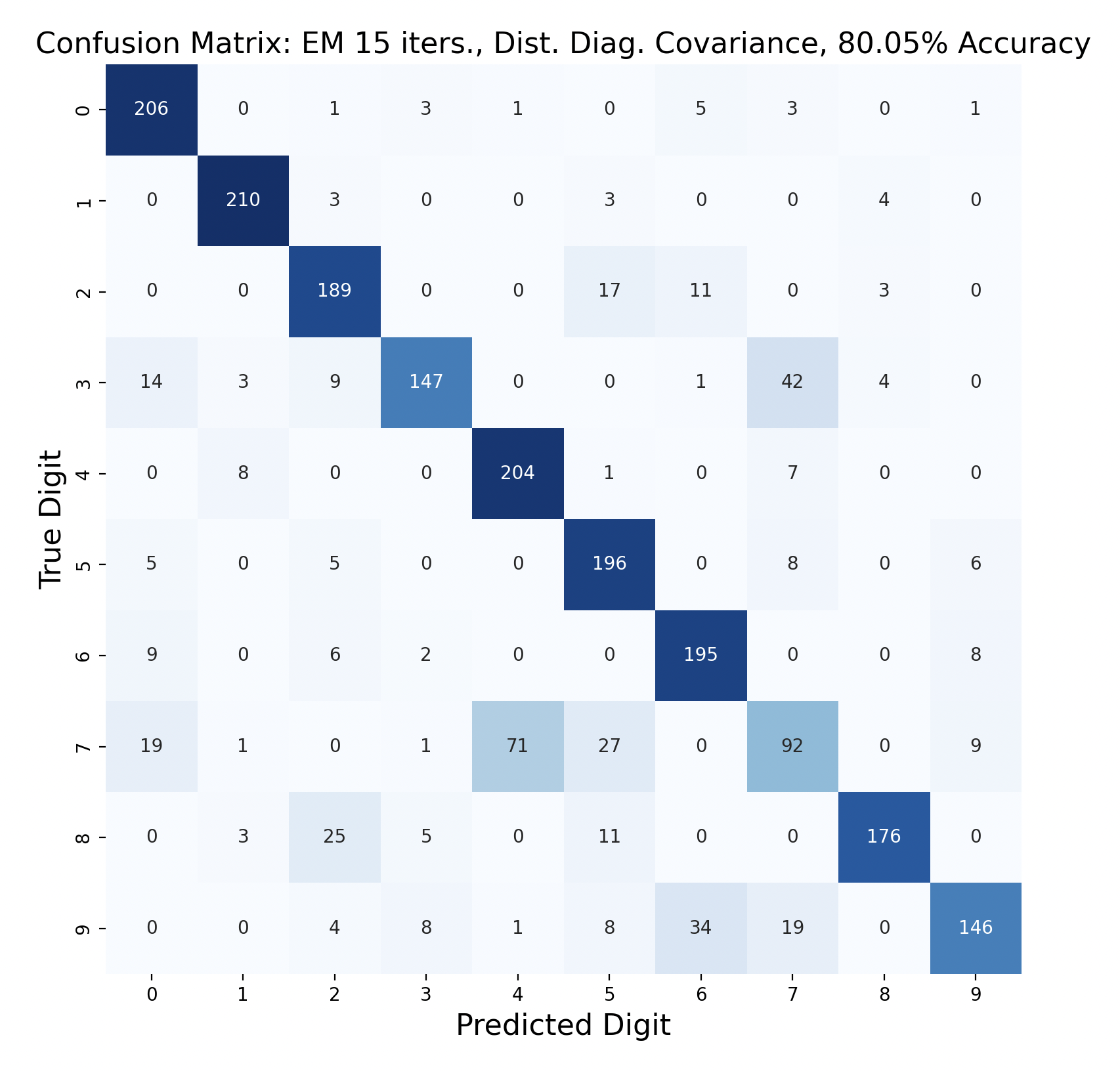
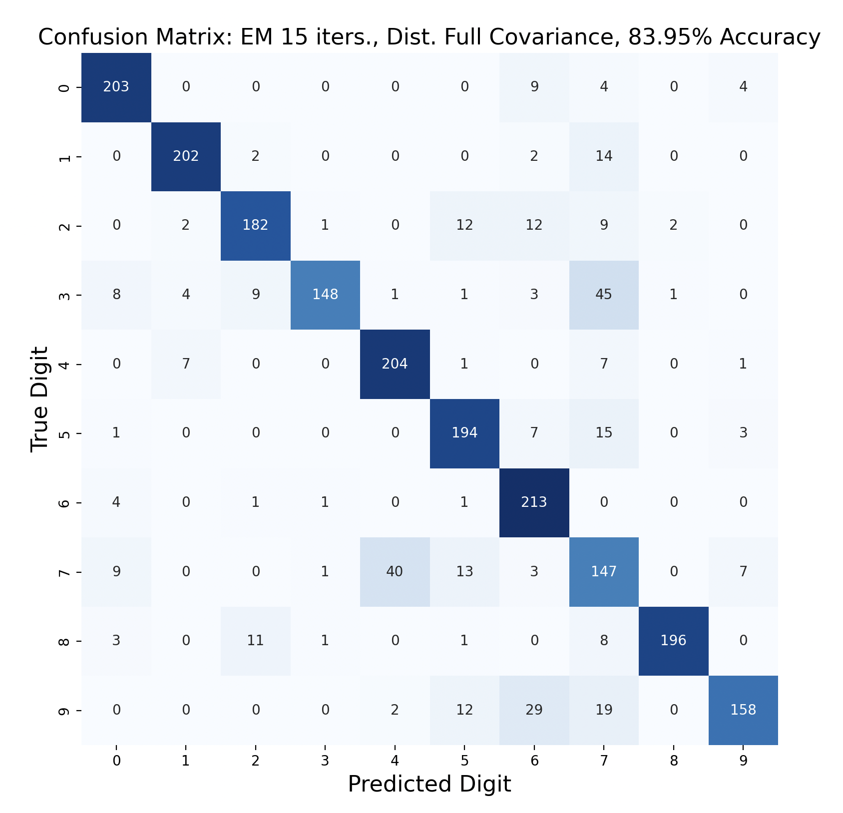
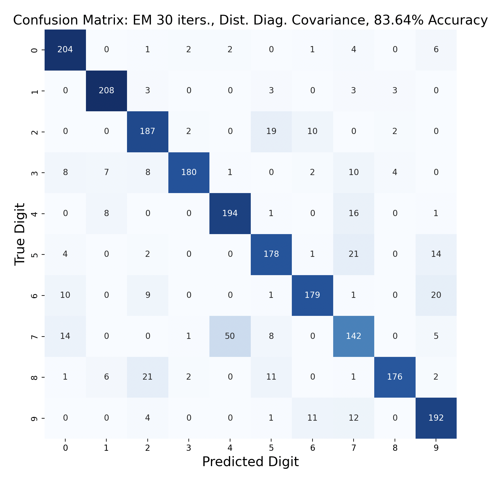
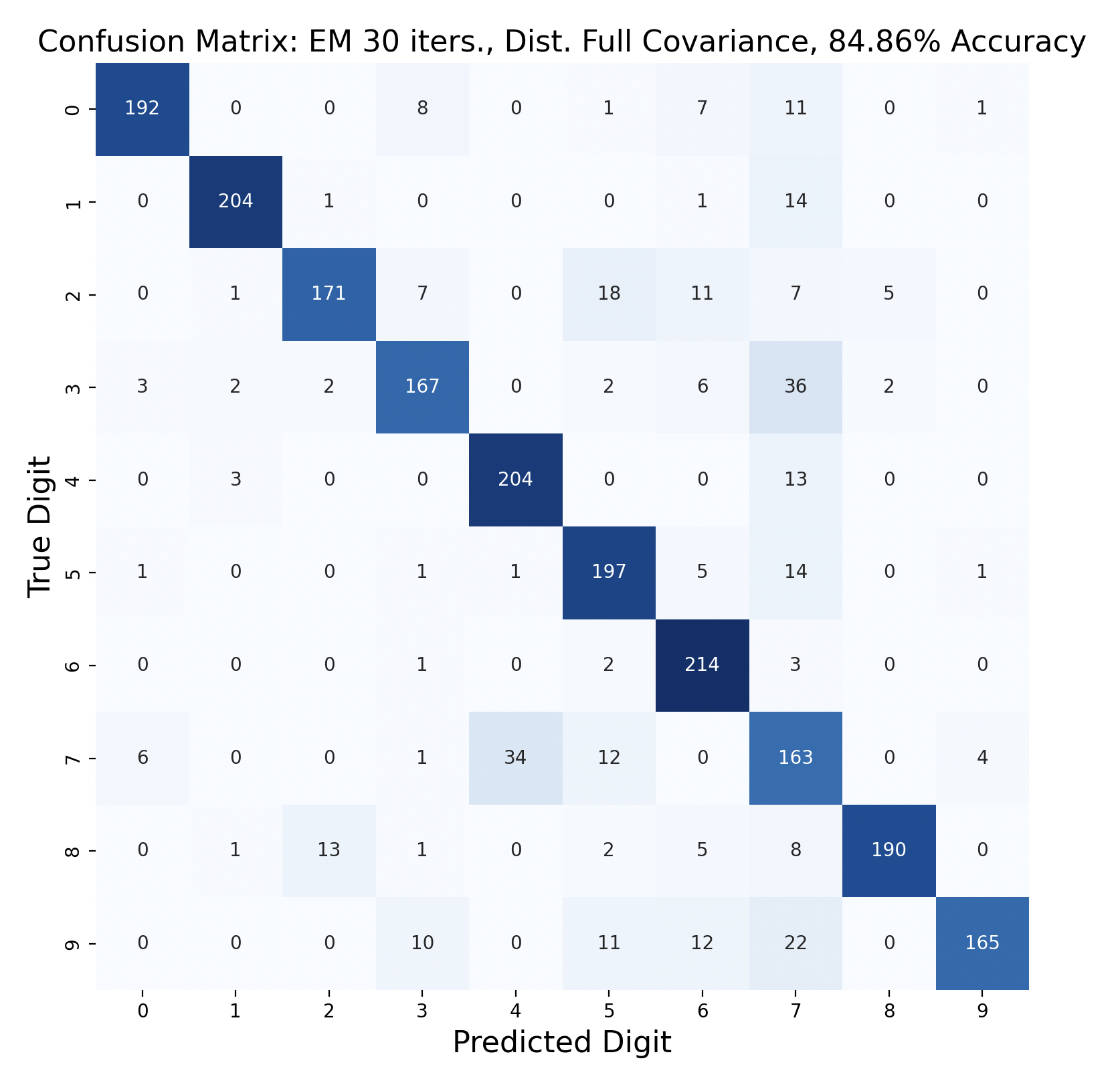
For three of the four EM tests, the k-means version with the same covariance and number of iterations performed better. This surprised me because I thought that EM would create more accurate GMMs. One explanation for this is that the Gaussians were fitted too closely to the training data, which resulted in lower accuracy. If this is the case, however, I would expect the full covariance to perform worse than the diagonal, since full covariance is closer to the shape of the data. For each number of iterations, full covariance matrices performed better.

The EM models had similar results for subproblems as k-means. One and six were accurately predicted throughout, and seven was often the least accurate. However, in both full covariance matrices predicting three as a seven was the most popular mistake. This mistake is less prevalent in the diagonal covariance models, so the difference in Gaussian shape must contribute to this occurrence.

The first challenge I faced when implementing maximum likelihood classification was breaking down the problem into code. Conceptually, the idea of finding the likelihood of a sample being all ten digits then choosing the maximum is straightforward, but due to the structure of the data this becomes more difficult. It became easier to solve the problem when thinking about what it would mean for a single frame to belong to a cluster, and then scaling this computation for all of the testing data.

One challenge I faced in implementing maximum likelihood classification for EM was the time it took to run trials. EM is significantly more computationally intense than k-means, primarily due to the calculation of covariance matrices for each cluster.

Another challenge was avoiding underflow. Underflow is an issue in computation that arises when very small numbers (much less than one) are multiplied and end up being expressed as zero, since computers cannot represent infinitely small values. This causes problems because multiplying zero by any other value also yields zero, and the information is lost. In order to find the total likelihood of a sample being a certain digit, the maximum likelihoods of each frame being a cluster are multiplied together, which can cause underflow. The solution to this problem is to use the log of the likelihood. This allows the log of the maximum likelihoods for each frame to be added together, and underflow is no longer an issue.

Conclusions

From my data modeling, I found the most important modeling choice to be the type of covariance matrix used in both k-means and expectation-maximization clustering problems. The covariance matrix defines the shape of the cluster Gaussians, which greatly impacts the likelihood that test data fits into each cluster. With less complex covariance types, this can hurt the model accuracy. Flexible covariance types might have a 10% boost in accuracy compared to rigid covariance matrices that make assumptions about covariance between variables (spherical and diagonal matrices). In addition, using distinct covariance matrices offers an accuracy advantage over tied covariance matrices, as cluster shapes can vary within digit GMMs.

The number of clusters, or k, is an important parameter for both k-means and EM. This parameter impacts both computation time and model accuracy, as four clusters take on a much different shape over the data than three clusters, which leads to different likelihood estimates and predictions. The more clusters that there are, the longer it takes to train the model, especially with EM as covariance is calculated each iteration for each cluster.

Surprisingly, the choice between k-means and EM did not matter as much as I expected it to. Assuming that enough iterations of the clustering algorithm were run to reach convergence, the difference in accuracy between k-means and EM models with the same covariance is not very large. In fact, k-means often outperformed EM for the same covariance and number of iterations.

Another less important choice is starting parameter values. Whether cluster means are random or even set to zero at first, the k-means algorithm, with enough iterations, is able to shift the means to become effective representatives of the model clusters. With EM, covariance can also be initialized arbitrarily, with the iterative updating of the parameters fixing incorrect assumptions about the data. One parameter that does matter a bit more is actually the probability. This is because probability multiplies the Gaussian in EM to get the likelihood for a frame being in a certain cluster. If probability is initialized to zero, the likelihood will always be zero. Using log likelihood, the log of zero is undefined, and log of an infinitesimally small number gives negative infinity. This means that the likelihood predictions for all frames would be artificially small and the resulting model would not be very accurate.

If I were to choose a single system to perform spoken digit recognition, I would use k-means clustering algorithm and perform maximum likelihood classification with distinct full covariance matrices. Throughout my testing, this model performed the most accurately and took much less time to train to convergence compared to EM. Training to convergence would take about 75 iterations.

This system is useful because it is relatively fast to compute – covariance matrices only need to be calculated after k-means is complete. Additionally, the least-accurate digit in the model, seven, has a prediction accuracy of 74.09%. The next least-accurate digit has an accuracy over 80%, so across all digits the model is consistent. The most common mistake in this model is predicting seven as four, so I would experiment with changing the kind of covariance matrix specifically for the GMM for seven, or with altering the probability for that GMM.

Throughout this process, I wrote code in several environments. I wrote several functions for calculating covariance and means that could be used across scripts, but in the future I would spend more time writing modular code, specifically for the clustering algorithms, so that it is easier to experiment with model changes. I found python notebooks to be significantly easier than python scripts because of the ability to run chunks of code rather than an entire file at once. This made testing the full system faster because I could edit code for maximum likelihood classification while keeping cluster assignments from k-means and EM. In the future, I would write all of my code in one environment and maintain modular functions whenever possible so that it is easy to try new things with my code.

Another lesson I learned was to make clean, readable plots that are labeled correctly. I often had to scrap a series of plots because the title and axis fonts were too small, or I forgot to add a legend for different sets of data. Next time, I will experiment with plot sizing and appearance in my portfolio before gathering the rest of the plots.

One choice I made throughout the project was to write my own clustering algorithms and functions to create covariance matrices. I tried to avoid packages in order to develop a stronger understanding of the entire machine learning process. This is something that I would continue in the future, as it also offers greater flexibility and control over the model, despite taking longer to implement. I think that the extra implementation time is worth fully understanding the algorithms.

References

Throughout this project I used modules for confusion matrices^[7], kernel density^[8], and multivariate normal distributions^[9] in my code. I also used the MathJax plugin^[10] to display mathematical formulas on my website.